고정 헤더 영역
상세 컨텐츠
본문
반응형
1. Overview
The principle of smoothing is to remove noise from the data by averaging several observations.
The smoothing method can be divided into a moving average method and a simple exponential smoothing method. Both methods (moving average, simple exponential smoothing) are suitable for time series in which there is no trend or seasonal variation.
Since the moving average method is easily used by many people, in this article, only the exponential smoothing method will be discussed.
The smoothing method is different from the moving average method in that it does not simply calculate the average of n numbers, but uses a weighted average of past data. The weights used to calculate the weighted average appear in the form of an exponential distribution.
That is, the most recent data is given the greatest weight, and the weight that decreases in the form of an exponential distribution is given as it goes into the past. Note that even the oldest observations are given a small weight.
To use the exponential smoothing method, a smoothing constant must be specified.
The smoothing constant is a parameter that controls how much weight is given to the past data when forecasting. If a smoothing constant value close to 1 is used, a greater weight is given to the recent observations when forecasting. Conversely, if a smoothing constant close to 0 is used, the past gives a greater weight to the value of
There is no specific method for determining the optimal smoothing constant, and sometimes the optimally obtained smoothing constant may lead to inaccurate results in predicting future data due to model overfitting. Therefore, a value between 0.1 and 0.2 is usually used.
2. Modeling
Holt-Winter's additive and multiplicative exponential smoothing methods can be used to predict seasonal data.
Holt-Winter's exponential smoothing method is characterized by considering seasonal variations within a specific period while forecasting after n periods.
It is suitable for time series with time level, trend, and seasonal component. Time level has Alpha, trend has Beta, and seasonal component has Gamma value.
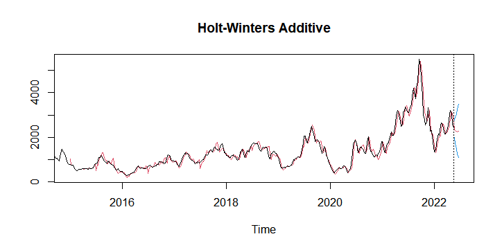
1) Holt-Winter additive model : When seasonality is constant regardless of the passage of time, additive model is used
| Date | Forecast |
| ‘22/24W(6/13~17) | 2,376.333 |
| ‘22/25W(6/20~24) | 2,308.458 |
| ‘22/26W(6/27~7/1) | 2,267.797 |
2) Holt-Winter multiplicative model: use multiplicative model when seasonality gradually increases variance with time
| Date | Forecast |
| ‘22/24W(6/13~17) | 2,348.397 |
| ‘22/25W(6/20~24) | 2,214.453 |
| ‘22/26W(6/27~7/1) | 2,186.486 |

3. Conclusion
Since the BDI time series graph has trend and seasonality, exponential smoothing is used, and among them, the additive model is used for future analysis.
728x90
'Forecast' 카테고리의 다른 글
| BDI & SCFI prediction (‘22/26W) (0) | 2022.06.26 |
|---|---|
| BDI & SCFI prediction (‘22/25W) (0) | 2022.06.19 |
| BDI & SCFI prediction (‘22/24W) (0) | 2022.06.12 |
| BDI & SCFI prediction (‘22/23W) (0) | 2022.06.05 |
| BDI & SCFI prediction (‘22/22W) (0) | 2022.05.29 |


댓글 영역